Fast Robots

Lab 10 - Simulator:

In this lab I setup and gained experience with the FlatLand simulator environment, which will be used for modelling robot control and localization in the next few labs. I also implemented simple closed loop collision avoidance functionality.

Simulator:

The FlatLand simulator developed for this course simulates the behavior of our robots from labs 1-9 but in a simplified, 2D environment. It consists of two parts, the simulator and the plotter. Both of these elements are controlled by the python Commander class. Functionality for the simulator includes setting robot velocity (both linear and angular), getting true pose and sensor values, and resetting the robot to its initial position. The simulator runs a GUI showing the robot in an environment replicating the one set up in lab. Thus the simulator can replicate the behavior of our robots in a simplified environment and produce both sensor measurements and ground truth values for comparison. The plotter can produce a solid line map replicating the physical robot environment set up in lab and plot XY points in three colors: red for odometry, green for ground truth, and blue for belief. Thus the plotter can be used to conveniently compare the true and calculated values of robot location in context with the map the robot is operating in.

Simulator GUI at initial position:

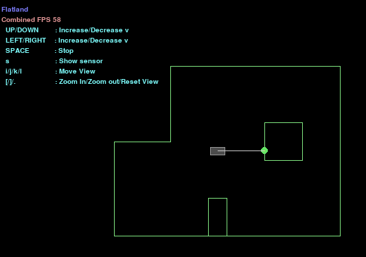
The small grey rectangle is the robot and the line protruding from it represents it's front TOF beam.

Open Loop Control:

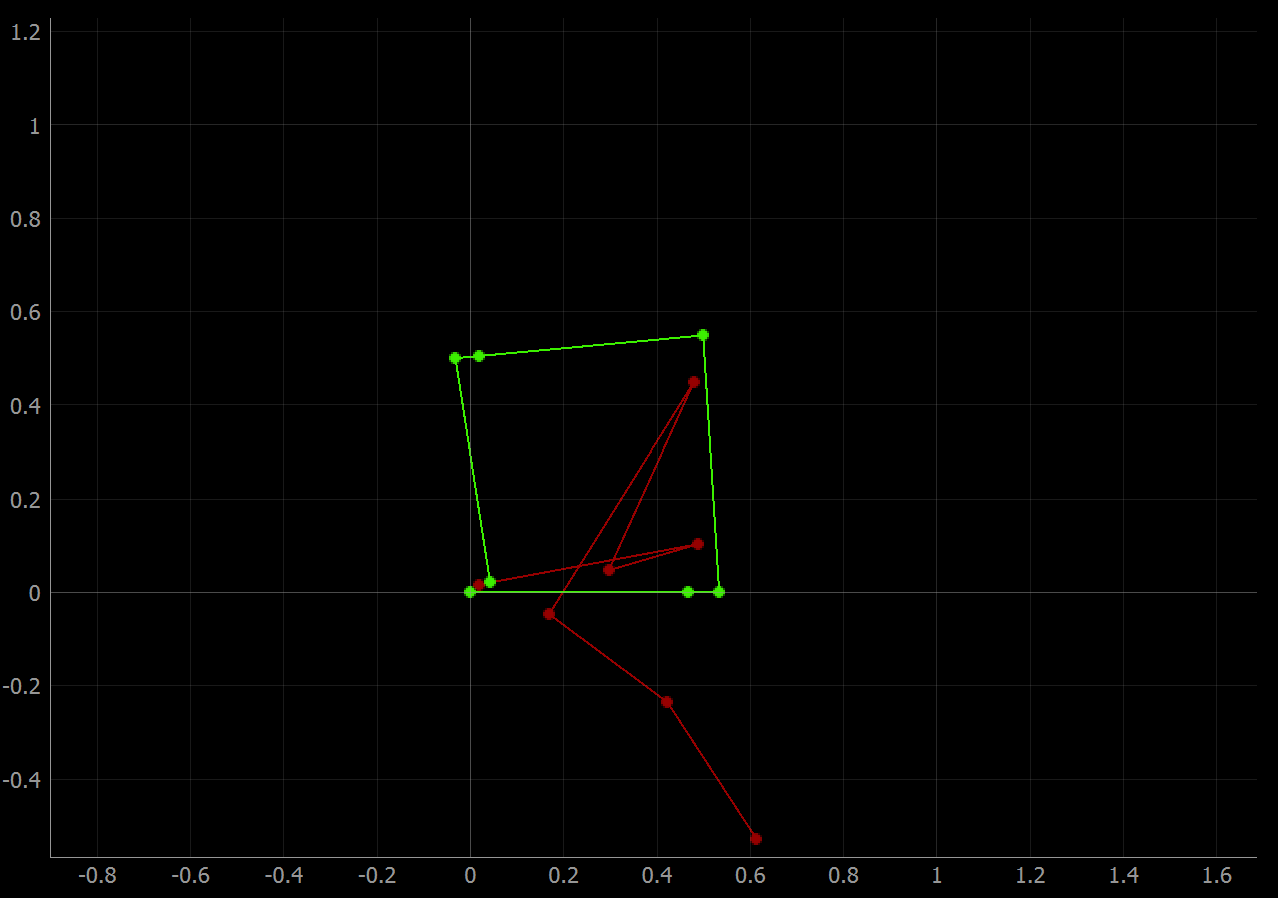
For this part of the lab, I designed a simple procedural algorithm to make the simulated robot move in a square pattern. At each corner of the square I plotted odometry and ground truth data. The procedure was to move straight at 1 m/s for 0.5 seconds, then stop and turn at 1rad/s for approximately pi/2 seconds. This was repeated four times, once for each edge of the square. Below is my procedural code, a screen recording of the simulated car moving, and the plotter output it generated.

Code for open loop control:

def plot_pose():
            pose, gt_pose = cmdr.get_pose()
            cmdr.plot_odom(pose[0], pose[1])
            cmdr.plot_gt(gt_pose[0], gt_pose[1])

        cmdr.set_vel(1,0)
        plot_pose()
        await asyncio.sleep(0.5)
        cmdr.set_vel(0,1)
        plot_pose()
        await asyncio.sleep(1.6)

        cmdr.set_vel(1,0)
        plot_pose()
        await asyncio.sleep(0.5)
        cmdr.set_vel(0,1)
        await asyncio.sleep(1.6)

        cmdr.set_vel(1,0)
        plot_pose()
        await asyncio.sleep(0.5)
        cmdr.set_vel(0,1)
        plot_pose()
        await asyncio.sleep(1.6)

        cmdr.set_vel(1,0)
        plot_pose()
        await asyncio.sleep(0.5)
        cmdr.set_vel(0,1)
        plot_pose()
        await asyncio.sleep(1.6)
        

The Commander set_vel(lin_v, ang_v) function moves the car for a theoretically infinite duration. It sets the linear and angular velocity to values lin_v in m/s and ang/v in rad/s and leaves the car in that state until the next time set_vel is called or until the car hits a wall. In order to make the car move for a limited time, I used the asyncio sleep function between calls of set_vel.

Video of open loop motion:

The simulated robot moves imperfectly with slight inconsistencies in movement durations, despite the fact that each call to asyncio.sleep is identical for a given motion (turning or moving along an edge).

Pose Plot 1: (green is ground truth, red is odometry)

Pose Plot 2: (same exact code as the first run)

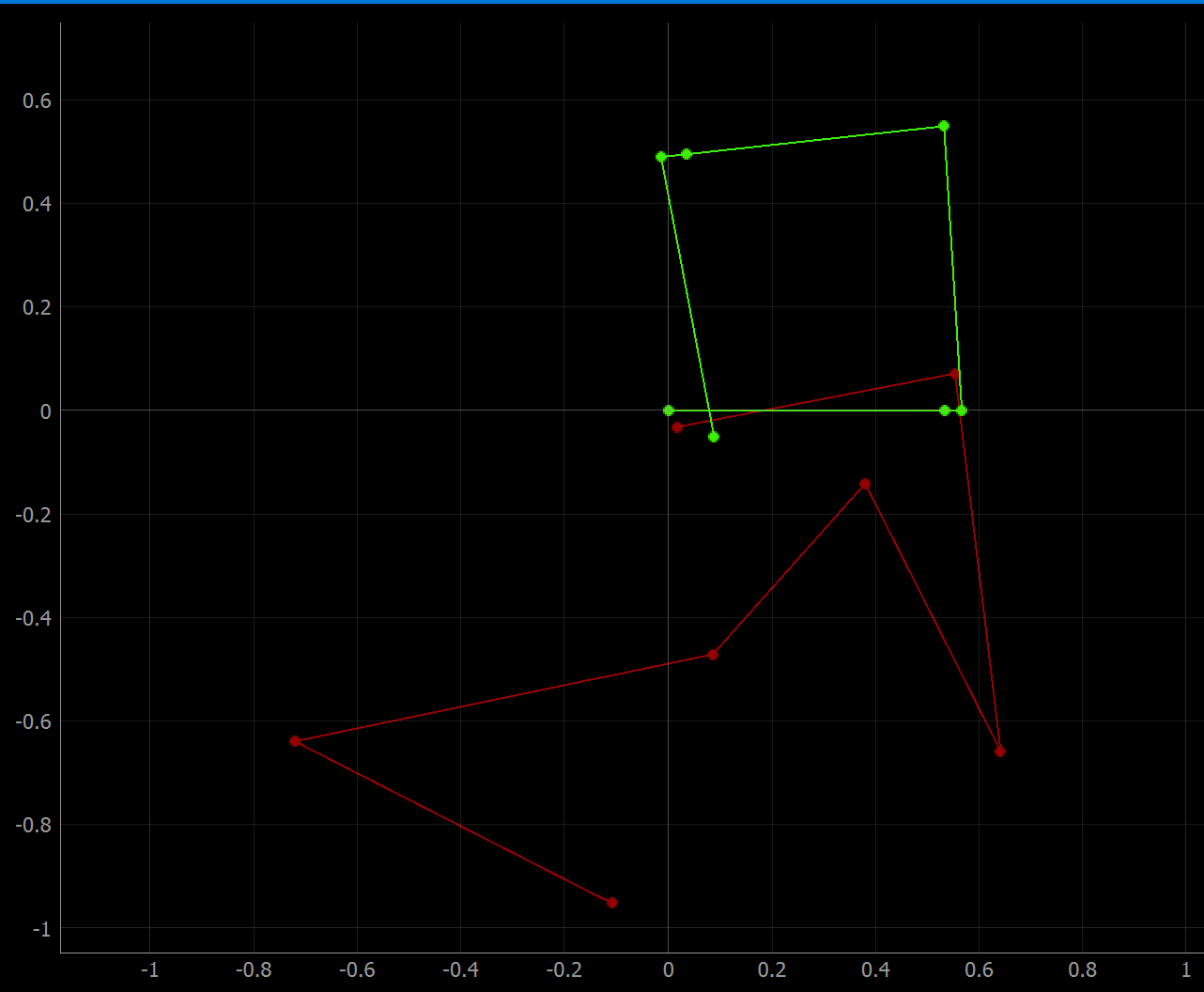
From the pose plots, it is clear that the robot's odometry in red, which simulates IMU data, does not present an accurate depiction of where it actually is. True location is given in green as the ground truth. This inaccuracy is due to snowballing accumulation of error in the integration needed to obtain position from IMU accelerometer and gyroscope data. Further, on multiple trials of the open loop control slightly different shapes were formed, likely due to inconsistencies in execution, especially in the use of asyncio.sleep which is device specific.

Closed Loop Control:

The next step in the lab is to code closed loop control obstacle avoidance for the simulated robot. To do this I went through several iterations using the front TOF sensor as input. This input is accessed through the Commander get_sensor function. First, I tried a simple algorithm where the robot would turn away from walls ahead in proportion to how close the wall is to the robot. The code was as below:

Code for initial closed loop control:

cmdr.set_vel(0.5, 0)

            while cmdr.sim_is_running() and cmdr.plotter_is_running():
            sensor_values = cmdr.get_sensor()
            plot_pose()
            if sensor_values[0] < 1:
                cmdr.set_vel(0.5, 3-sensor_values[0])
        

This worked decently well, but had one major flaw. The beam of the simulated front tof sensor is extremely narrow, far more narrow than the robot itself. With the above algorithm, the robot moved straight except for when it perceived a nearby wall. So when using this control system, the beam could narrowly miss a wall which caused the robot to believe it had a safe path forward. Then the edge of the car would collide with an obstacle. To solve this, I decided the robot should oscillate back and forth while moving and turn toward whichever direction showed a greater distance to an obstacle. That way, rather than glancing off of obstacles that are narrowly off center from it, it would oscillate towards them, see a small distance, and turn away. Below is a the code used, a screen capture of this control system in action and a plot of the pose output.

Code for final closed loop control:

osc = 2
        last_tof = 1

        cmdr.set_vel(0.5, 0)
        
        while cmdr.sim_is_running() and cmdr.plotter_is_running():
            sensor_values = cmdr.get_sensor()
            plot_pose()
            if sensor_values[0] < 1:
                cmdr.set_vel(0.5, 3-sensor_values[0])
            elif sensor_values[0] < last_tof: 
                cmdr.set_vel(0.5, -1*osc)
            else:
                cmdr.set_vel(0.5, osc)
            osc *= -1
            last_tof = sensor_values[0]
        

The functionality from the initial control code iteration is maintained because it was effective at avoiding walls when they were sensed nearby. However, rather than simply going straight when no walls are in front, the car searches for obstacles in its path. The osc value switches back and forth, and at each oscillation the front sensor value is taken and stored. When there is a change the car tends to turn toward an obstacle, which is actually helpful in making the obstacle avoidance from above work because the obstacle is sighted.

Video of closed loop motion:

Success! This was taken with a linear velocity of 0.5 m/s.

Pose Plot: (green is ground truth, red is odometry)

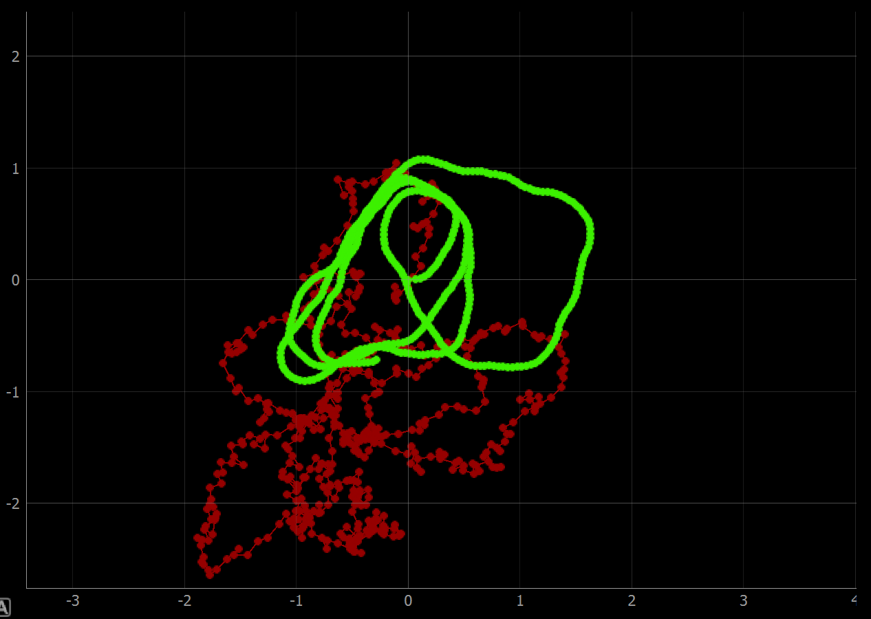
From this plot it can be seen that the robot traversal of the maze was stable and covered all areas of the map.

Faster linear velocity:

This is the car moving at 0.75 m/s. It does a decent job avoiding obstacles but eventually collides due to not having time to turn away from a wall after sensing it late.

Pose Plot:

The robot successfully traversed the whole map but eventually collided at a corner. To guarantee collision avoidance the control should be run at a speed of 0.5 m/s or less.