Lab 7 - Kalman Filter:
In this lab I implemented a Kalman filter for obtaining a faster and more accurate estimation of the robot's position. The KF incorporated the prior belief and motion of the robot with sensor data in a probabilistic model to find the robot's state.
Motion Model/Step Response:
To determine a valid motion model of the robot, I ran data collection on a motor step response and solved for matrix coefficients to be used in the model. Based on Newton's second law and the general equation for drag force, I estimated the motion model to be of the form:
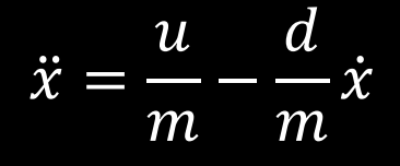
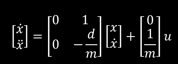
This yields the following state space equation:
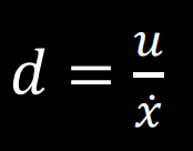
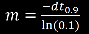
To calculate the drag and mass coefficients, I ran a motor step response by setting the motors to 90% drive (PWM of 96.5) for the span of 60 TOF measurements. Then, I calculated the drag using the steady state velocity and mass using the 90% rise time according to the below formulas:
Below are plots of the motor input, position (by TOF data), and velocity (by differentiating TOF data) of the robot during the step response.
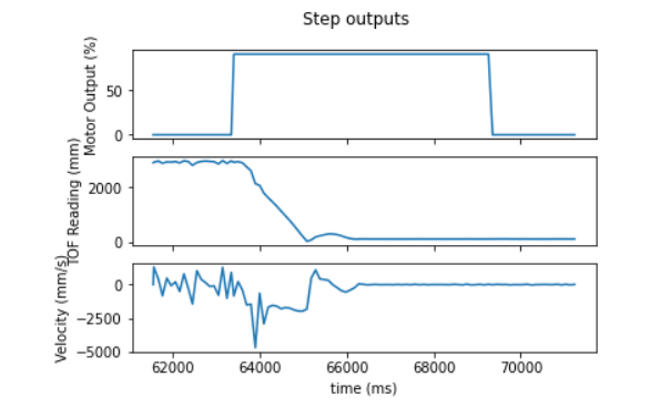
From this data, I found that the steady state velocity was 1800 mm/s and the 90% rise time was 0.79 s. Thus, using the formulas above I calculated the value of the mass coefficient to be 1.91x10^-4 and that of the drag coefficient to be 5.6x10^-4 when normalizing the input u to 1. These values result in the following state space matrices:
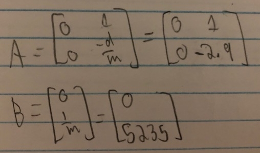
All remaining motion model matrices (the C matrix and noise matrices) are the same as calculated in lecture and are as follows:

Implementing a Kalman Filter on Lab 6 data:
To sanity check my KF, I implemented it in Python and ran it on data collected during Lab 6. Below is my code to make that happen.
Delta_T = time_stamps[3]-time_stamps[2]
        # taken from middle because more representative than first time step

        A = np.array([[0,1],[0, -2.9]])
        B = np.array([[0], [5235 / 1000]])
        C = np.array([[-1,0]])

        sigma_u = np.array([[100, 0],[0,100]])
        sigma_z = np.array([[400]])

        Ad = np.eye(2) + Delta_T * A
        Bd = Delta_T * B


        ARR_SIZE = len(tofs)

        step_size = 43.5 # lab 6 final version max motor output percentage. Scales to 56.975 PWM.

        def kf(mu,sigma,u,y):
            #prediction
            mu_p = Ad.dot(mu) + Bd.dot(u)
            sigma_p = Ad.dot(sigma.dot(Ad.transpose())) + sigma_u

            #update
            y_m = y-C.dot(mu_p)
            sigma_m = C.dot(sigma_p.dot(C.transpose())) + sigma_z

            kf_gain = sigma_p.dot(C.transpose().dot(np.linalg.inv(sigma_m)))

            mu = mu_p + kf_gain.dot(y_m)
            sigma=(np.eye(2)-kf_gain.dot(C)).dot(sigma_p)
            return mu,sigma

        #initial values
        kf_x = np.array([[-tofs[0]],[0]])
        sigma = np.array([[25,0],[0,25]])

        kf_results = []
        for i in range(ARR_SIZE):
            kf_x, sigma = kf(kf_x,
                            sigma,
                            [[motor_pcnts[i] / step_size]],
                            np.array([[tofs[i+1]]]))
            dist = -kf_x[0,0]
            kf_results.append(dist)
The KF function is based on the one provided in our lab manual. It uses my motion model established above to predict the location of the robot, then fuses that prediction with sensor data in order to generate a new position and noise estimate for the robot's state. This function is called iteratively on every TOF and motor drive value from Lab 6. My Lab 6 implementation only recorded motor percentages along with TOF values, so the arrays containing these values are corresponding and of the same size. Running this KF simulation yielded the following data result:
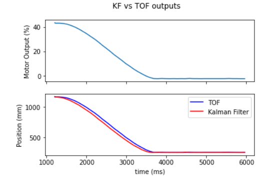
From these graphs, I inferred that the KF I implemented follows the TOF values fairly closely, but anticipates a faster approach based on the car's motion model. This is useful because it allows me to run the car at faster speeds, which the slow TOF measurements can't keep up with, and the KF will account for this and give a more up to date position estimate.
Implementing a Kalman Filter on the robot:
Now, in order to put the KF to use, I translated the code to Arduino and ran it live on the robot while in motion. I used the Arduino BasicLinearAlgebra library for matrix operations and fed the position outcome of the KF into my preexisting PID function from lab 6 for motor control. The code I used is as follows:
KF function:
///////KALMAN FILTER////
            Matrix<2,2> A = {0, 1,
            0, -2.9};
        Matrix<2,1> B = {0, 5.235};
        Matrix<1,2> C = {-1, 0};

        Matrix<2,2> sigma_u = {100, 0,
                0, 100};
        Matrix<1> sigma_z = {400};

        Matrix<2,2> I = {1, 0,
        0, 1};

        #define STEP_SIZE 43.5

        float kf(int index, long time_stamp, int tof_dist){
        if (index == 0){
        //store initial values
        Matrix<2,1> mu = {tof_dist, 0};
        Matrix<2,2> sigma = {25,0,
                    0, 25};
        store_kf_data(index, mu, sigma);
        return mu(0,0);
        }

        // Get KF inputs for this iteration
        Matrix<2,1> mu = kf_vals[index-1];
        Matrix<2,2> sigma = sigmas[index-1];
        Matrix<1, 1> u = {motor_pcnts[index-1] / STEP_SIZE};
        Matrix<1> y = {tof_dist};
        int dt = time_stamp - times[index-1];
        Matrix<2,2> Ad = I + A * dt;
        Matrix<2,1> Bd = B * dt;

        //predict step
        Matrix<2,1> mu_p = Ad * mu + Bd * u;
        Matrix<2,2> sigma_p = Ad*sigma*~Ad + sigma_u;

        //update step
        Matrix<1> y_m = y - C * mu_p;
        Matrix<1,1> sigma_m = C * sigma_p * ~C + sigma_z;

        Matrix<1,1> sigma_m_inv = sigma_m;
        Invert(sigma_m_inv);
        Matrix<2,1> kf_gain = sigma_p * ~C * sigma_m_inv;

        //combine
        mu = mu_p + kf_gain * y_m;
        sigma = (I - kf_gain * C) * sigma_p;

        store_kf_data(index, -mu, sigma);
        return -mu(0,0);
        }
The constant matrix coefficients are initialized at the top. The Kalman Filter relies on past TOF and motor percent values, so on the first function iteration it simply accepts the first TOF value as position, assumes velocity is 0, and establishes a reasonable initial uncertainty. Then in future iterations the function establishes KF parameters specific to the current TOF data, previous KF state and previous motor input, predicts state with the motion model, updates with TOF data, and returns current position. It returns current position for use by the PID controller in controlling the motors. KF position, velocity, and uncertainty are used in future iterations of the controller though and are saved using store_kf_data.
Outer loop logic:
 if(sensor_data_ready() && measure_count < ARR_SIZE){
            //Doing KF and just got new sensor reading
            curr_mil = millis();
            new_tof = get_front_tof();
            kf_state = kf(measure_count, curr_mil, new_tof);
            pcnt = pid(measure_count, curr_mil, kf_state, new_tof);

            move_speed(pcnt);
            measure_count ++;
            }
            else if (measure_count >= ARR_SIZE){
            active_stop();
            write_pid_data();
            write_kf_data();
            do_KF = false;
            }
The outer loop calls the KF function which fuses sensor data, information of prior motor execution, and prior KF belief to estimate robot position. This position is fed into the PID controller, which controls the motors and records the motor percentage and TOF data. This happens for 100 cycles, at which point the KF position data, TOF readings, and motor percentages are written to BLE and sent to a lab computer for analysis. Below are graphs of the output from one run of the Kalman Filter.
KF Results:
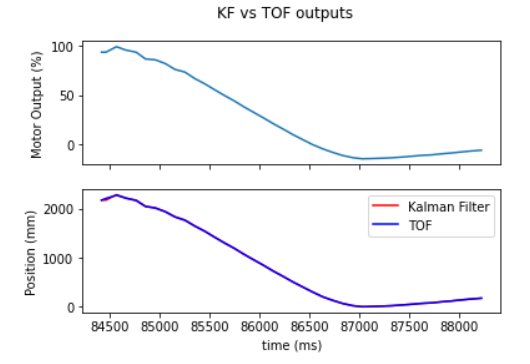
The KF data was very close (but not identical) to the TOF data, which indicates that my Kalman Filter places a high level of a confidence in sensor values. However, the trial was a success, placing the robot 300mm away from the wall without collision. It also was run using significantly more aggressive PID parameters and motor scaling than in lab 6 and ran far faster. See below video: