Lab 9 - Mapping:
In this lab I collaborated with David Kim (jk2537) to create a map of the provided robot environment using the proximity sensors on our robot. We were set several points in the environment to place the robot and allow it to rotate, collecting TOF sensor data. This data was then processed and combined into a map of the environment.
Control:
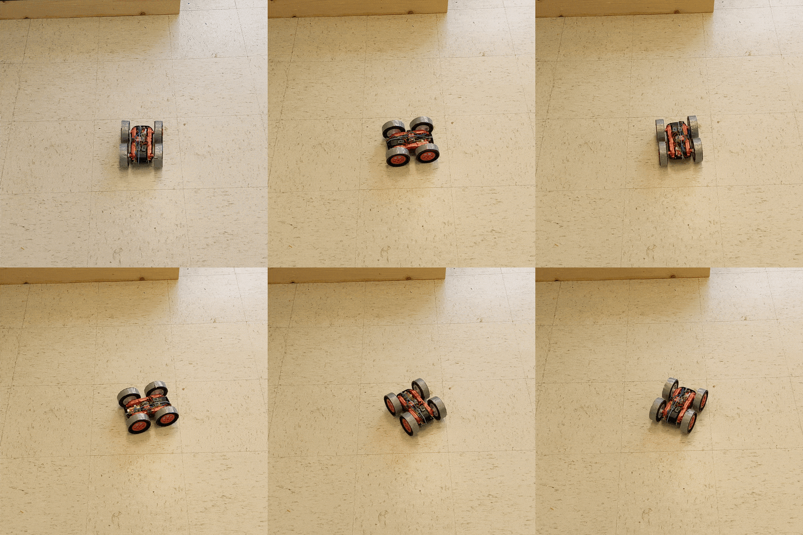
At first, we tried to implement PID velocity control to rotate the car, using a setpoint of 15 radians per second. We planned to integrate the resultant gyroscopic angular velocity data to find the orientation of the robot. However, we quickly found several issues with this method. Our gyroscopic data was inconsistent and irregular and the car was unable to turn on its axis at a sufficiently slow pace to enable sufficient TOF sensing. However, we did notice that when providing a high velocity setpoint in periodic start-stops, we were able to reliably achieve a 360 degree turn in 14 even rotations, collecting 15 data points. Therefore, we switched to using orientation control taking 15 points evenly spaced over a full turn.
Video of car rotating:
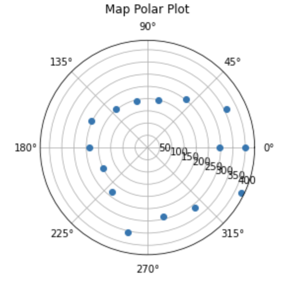
Plot of output when rotating in square, walled off region:
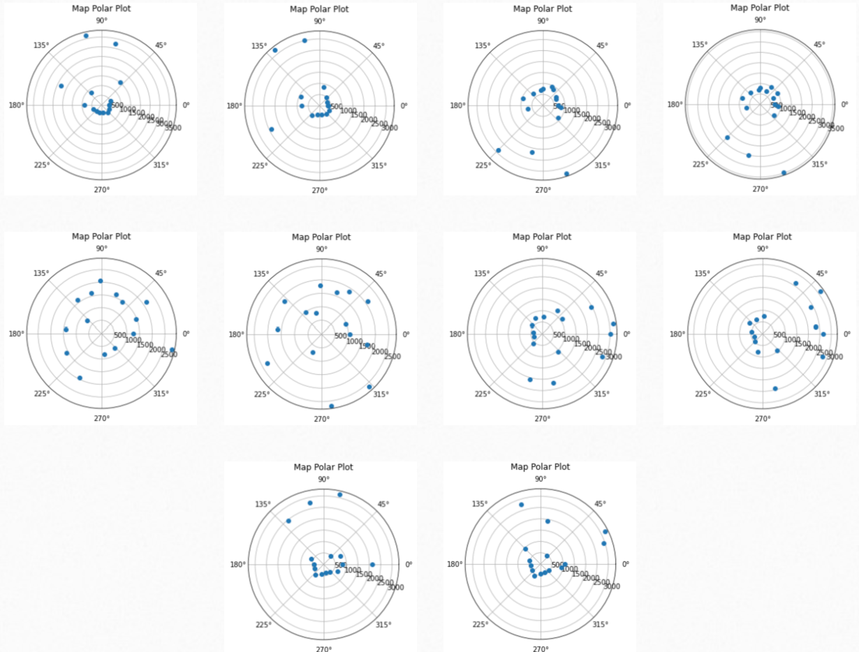
Next, we set the robot on given points in the provided map environment and collected measurements. Below are polar plots of the TOF readings we received versus orientation.
XY Conversion:
These distance readings were converted to points on an XY axis using basic trigonometry. However, some data had to be rotated due to accidental inconsistencies in the initial orientation of the robot during data collection.
Merge Plot:
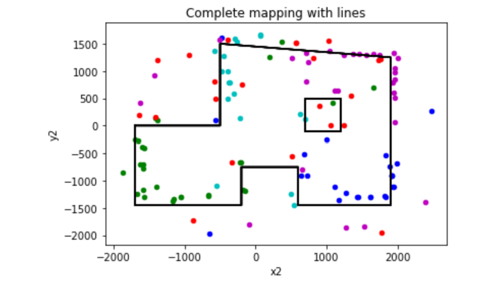
In order to make this data useful, it needs to be combined and transformed onto a reference frame representing the entire room. To combine the data, first each set of XY data in millimeters is translated to originate at its respective scan spot. The XY locations of the spots are converted to millimeters using 1ft = 304.8mm and added to the sensor XY data. Next, the data was filtered to only include points within a reasonable range, in this case within 2 meters of the global origin. The resultant data, with points colored by scanning spot, is below.
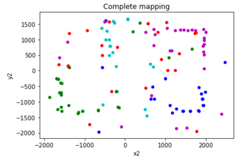
Finally, I manually added lines to the plot to create a finished map. This map is imperfect, but definitely shows the general layout of the environment. It could be improved with more points and a more advanced control method.
